Retarded Green’s Function
This tutorial shows how to compute the retarded Green’s function using a custom quantum circuit (CFusion) and compare it with the exact result.
We will go through the following steps:
Define system parameters and lattice Hamiltonian
Construct a variational quantum circuit as the ground state
Evaluate the retarded Green’s function
Compare with exact solution
Visualize the results
[1]:
import numpy as np
from c_fusion import CFusion

from isqham.greenfunction.retardedGreenfunction import RetardedGreenFunction
from isqham.lattice.fermionLattice import Gt_exact, getLatticeHam

U = 3.0
N = 60

tMax = 30
tN = 100


latHam = getLatticeHam(U=U)


def optimized_phi(t, U, V):
    alpha = (U - V) / 4
    beta = (t**2 + alpha**2) ** 0.5
    sin = (alpha - beta) / (((alpha - beta) ** 2 + t**2) ** 0.5)
    phi = -np.arcsin(sin) * 2
    return phi


phi0 = optimized_phi(t=-1, U=U, V=0)


def get_gs():

    gs = CFusion(4)
    gs.RY(0, phi0)
    gs.CNOT(0, 1).CNOT(1, 2).CNOT(2, 3)
    gs.Y2M(0)
    gs.X(1).X(3)
    gs.CNOT(0, 1).CNOT(1, 2).CNOT(2, 3)
    return gs


gs = get_gs()

gt = RetardedGreenFunction(
    H=latHam, N=N, circuit_cls=CFusion, ground_state=gs, shots=1024
)

i = 0
j = 0
Tlist = np.arange(0, 25, 0.1)
GT = gt.G(i=i, j=j, Tlist=Tlist)

exc_gt = Gt_exact(U=U, i=i, j=j)
GT_ex = np.array([exc_gt.get(t=t) for t in Tlist])
[2]:
import matplotlib.pyplot as plt
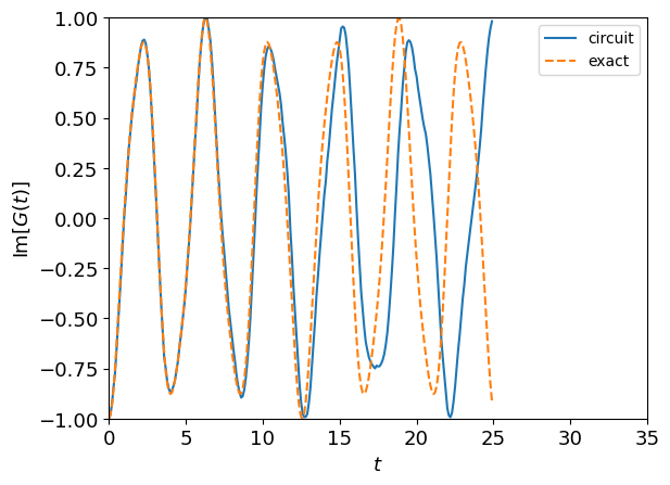
def fig2_GT_result(ax):
ax.plot(Tlist, GT.imag, "-", label="circuit")
ax.plot(Tlist, GT_ex.imag, "--", label="exact")
ax.set_ylim([-1, 1])
ax.set_xlim([0, 35])
ax.set_ylabel("$\\text{Im}[G(t)]$", size=13)
ax.set_xlabel("$t$", size=13)
ax.tick_params(axis="both", which="major", labelsize=13)
ax.legend(loc="upper right")
ax = plt.gca()
fig2_GT_result(ax)
[3]:
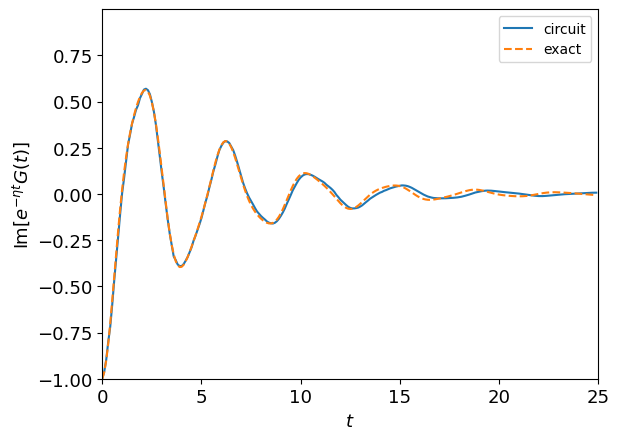
def fig2_GT_with_eta_result(ax):
    ax.plot(Tlist, GT.imag * np.exp(-0.2 * Tlist), "-", label="circuit")
    ax.plot(Tlist, GT_ex.imag * np.exp(-0.2 * Tlist), "--", label="exact")
    ax.set_ylim([-1, 0.9999])
    ax.set_xlim([0, 25])
    ax.set_ylabel(r"$\text{Im}[e^{-\eta t} G(t)]$", size=13)
    ax.set_xlabel("$t$", size=13)
    ax.tick_params(axis="both", which="major", labelsize=13)
    ax.legend()


ax = plt.gca()


fig2_GT_with_eta_result(ax)
[4]:
import matplotlib.pyplot as plt
import matplotlib.transforms as mtransforms
import numpy as np
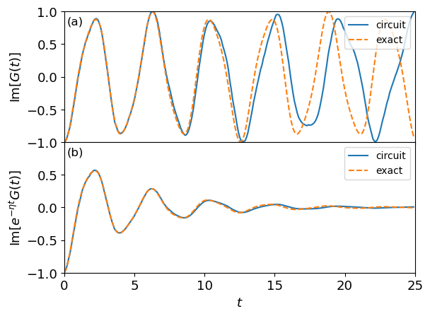
fig, axs = plt.subplots(2, 1, sharex=True)
fig.subplots_adjust(hspace=0)
trans = mtransforms.ScaledTranslation(10 / 72, -5 / 72, fig.dpi_scale_trans)
fig2_GT_result(axs[0])
fig2_GT_with_eta_result(axs[1])
axs[0].text(
-0.02,
1.0,
"(a)",
transform=axs[0].transAxes + trans,
fontsize="large",
verticalalignment="top",
)
axs[1].text(
-0.02,
1.0,
"(b)",
transform=axs[1].transAxes + trans,
fontsize="large",
verticalalignment="top",
)
plt.legend()
[4]:
<matplotlib.legend.Legend at 0x7fc7770d97f0>
[5]:
from isqham.greenfunction.frequencyGreenf import GreenFuncZ

gw_exact_omega = np.load("./docs/green_function/gw_eta0.2.x.npy")
gw_exact_gw = np.load("./docs/green_function/gw_eta0.2.y.npy")
gz = GreenFuncZ(tMax=tMax, tN=tN, rGObj=gt)
GW = gz.Gz(i=i, j=j, zList=gw_exact_omega + 0.2 * 1j)
[6]:
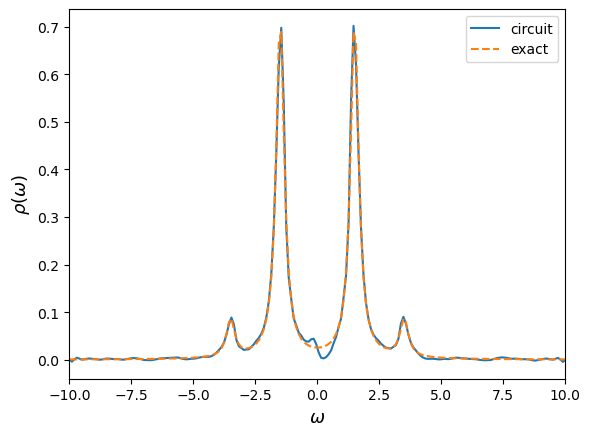
def fig2_GW_dos_result(ax):
    wList = gw_exact_omega
    gExact = gw_exact_gw
    ax.plot(wList, -GW.imag / np.pi, "-", label="circuit")
    ax.plot(wList, -gExact.imag / np.pi, "--", label="exact")
    ax.set_xlim([-10, 10])
    ax.set_ylabel(r"$\rho(\omega)$", size=13)
    ax.set_xlabel(r"$\omega$", size=13)
    ax.legend()


ax = plt.gca()
fig2_GW_dos_result(ax)
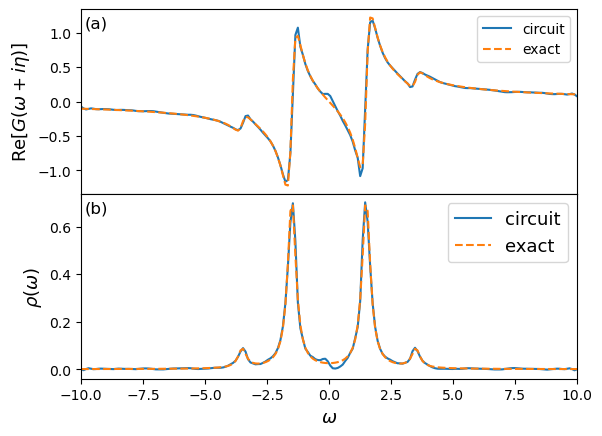
[7]:
def fig2_GW_real_result(ax):
    wList = gw_exact_omega
    gExact = gw_exact_gw
    ax.plot(wList, GW.real, "-", label="circuit")
    ax.plot(wList, gExact.real, "--", label="exact")
    ax.set_xlim([-10, 10])
    ax.set_ylabel(r"$\text{Re}[G(\omega+i\eta)]$", size=13)
    ax.set_xlabel(r"$\omega$", size=13)
    ax.legend()


ax = plt.gca()


fig2_GW_real_result(ax)

[8]:
import matplotlib.pyplot as plt
import matplotlib.transforms as mtransforms
import numpy as np


fig, axs = plt.subplots(2, 1, sharex=True)


trans = mtransforms.ScaledTranslation(10 / 72, -5 / 72, fig.dpi_scale_trans)


fig.subplots_adjust(hspace=0)


fig2_GW_real_result(axs[0])
fig2_GW_dos_result(axs[1])


axs[0].text(
    -0.02,
    1.0,
    "(a)",
    transform=axs[0].transAxes + trans,
    fontsize="large",
    verticalalignment="top",
)
axs[1].text(
    -0.02,
    1.0,
    "(b)",
    transform=axs[1].transAxes + trans,
    fontsize="large",
    verticalalignment="top",
)


# axs[1].tick_params(axis='both', which='major', labelsize=13)
plt.legend(fontsize=13, title_fontsize=15)
[8]:
<matplotlib.legend.Legend at 0x7fc778a5c110>
Appendix: Notes and References
This tutorial shows the use of quantum circuits to simulate Green’s functions.
For theoretical background, see:
Utilizing Quantum Processor for the Analysis of Strongly Correlated Materials