Retarded Green’s Function Calculation
This tutorial demonstrates how to compute the retarded Green’s function for a strongly correlated lattice model using the isqham library.
Objectives
Understand the structure of the lattice Hamiltonian.
Learn how to compute the time evolution of Green’s function.
Visualize the results with NumPy and Matplotlib.
[1]:
import numpy as np
from c_fusion import CFusion

from isqham.greenfunction.frequencyGreenf import GreenFuncZ
from isqham.greenfunction.LatticeGreen import LatticeGreenFunction
from isqham.greenfunction.retardedGreenfunction import RetardedGreenFunction
from isqham.lattice.fermionLattice import getLatticeHam, getSupH
[2]:
U = 3
N = 60

tMax = 30
tN = 100
eta = 0.2

supH = getSupH(U=U)
clusterH = getLatticeHam(U=U)


def optimized_phi(t, U, V):
    alpha = (U - V) / 4
    beta = (t**2 + alpha**2) ** 0.5
    sin = (alpha - beta) / (((alpha - beta) ** 2 + t**2) ** 0.5)
    phi = -np.arcsin(sin) * 2
    return phi


phi0 = optimized_phi(t=-1, U=U, V=0)


def get_gs():
    gs = CFusion(4)
    gs.RY(0, phi0)
    gs.CNOT(0, 1).CNOT(1, 2).CNOT(2, 3)
    gs.Y2M(0)
    gs.X(1).X(3)
    gs.CNOT(0, 1).CNOT(1, 2).CNOT(2, 3)
    return gs


gs = get_gs()

### set Green's function generator
gt = RetardedGreenFunction(
    H=clusterH, N=N, circuit_cls=CFusion, ground_state=gs, shots=1024
)
gz = GreenFuncZ(tMax=tMax, tN=tN, rGObj=gt)
latG = LatticeGreenFunction(GZ=gz, supH=supH)


OmegaMax = 6.0
Gamma = np.array([0.0, 0.0, 0.0])
X = np.array([0, np.pi, 0.0])
M = np.array([np.pi, np.pi, 0.0])
kPoints = [Gamma, X, M, Gamma]
Omega = np.arange(-OmegaMax, OmegaMax, 0.1)

rho = latG.getDensityOfState(
    kPoints=kPoints, OmegaPoints=Omega, eta=eta, kMesh=40, index=[0]
)
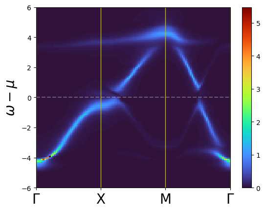
[3]:
import matplotlib.pyplot as plt

fig = plt.figure()
ax = plt.axes()

Xlablist = [r"$\Gamma$", "X", "M", r"$\Gamma$"]
extent = (0, len(Xlablist) - 1, -6, 6)

imsh = ax.imshow(
    rho, extent=extent, cmap="turbo", aspect="auto", vmin=0, vmax=rho.max()
)

bar = plt.colorbar(imsh)

ax.set_xticks(range(len(Xlablist)))
ax.set_xticklabels(Xlablist, size=20)
ax.set_ylabel(r"$\omega-\mu$", size=20)
ax.xaxis.grid(True, which="major", color="y", linestyle="-", linewidth=1)
plt.plot([0, 3], [0, 0], "--", color="w", alpha=0.3)
[3]:
[<matplotlib.lines.Line2D at 0x7f2b6d6c15e0>]
Appendix: Notes and References
This tutorial shows the use of quantum circuits to simulate Green’s functions.
For theoretical background, see:
Utilizing Quantum Processor for the Analysis of Strongly Correlated Materials