自动微分

1. 创建isQ代码

在一般的量子电路模拟中，我们建议使用sample=False，这种模拟方式可以得到量子电路精确测量结果（理论概率分布），而不用担心shots的问题。精确的模拟结果是shots趋向于无穷大的极限值。
当使用精确模拟时，还有一个好处是我们可以使用AutogradBackend, TorchBackend后台，解析求得参数的梯度。首先我们建立一个含有参数params[]的量子电路。

这段代码命名为gradient.isq，并且放在同一个目录。

import std;


param params[];
qbit q[1];

unit main() {
    Ry(params[0], q[0]);
    Rx(params[1], q[0]);
    M(q[0]);
}

2. 使用Autograd进行自动微分

Autograd作为numpy的轻量拓展，可以用来实现自动求导。首先，我们使用AutogradBackend作为后台模拟，sample=False得到精确模拟结果，使用numpy定义一个数组params1，定义一个函数circuit1。在该函数中，qc1.measure(params=params1)中以关键字参数的形式传入我们的参数。params=params1等号左边对应gradient.isq中参数的定义，等号右边对应着python中定义的数组params1。函数circuit1的返回值为测量结果数组中的第一个数results[0]。

from isqtools import IsqCircuit
from isqtools.backend import AutogradBackend, TorchBackend
import numpy as np


autograd_backend = AutogradBackend()

qc1 = IsqCircuit(
    file="gradient.isq",
    backend=autograd_backend,
    sample=False,
)

params1 = np.array([0.9, 1.2])

def circuit1(params1):
    results = qc1.measure(params=params1)
    return results[0]

print(circuit1(params1))

0.6126225961314372

此时使用autograd中的grad方法，对函数circuit1进行求导即可。grad可以传入需要求导的参数的编号索引作为第二个参数，在这里，由于circuit1函数只有一个参数params1，因此可以传入[0]作为需要求导的序号。grad返回一个Callable对象，传入参数即可得到对于参数的导数。更多的额用法请参考Autograd的官方网站。

from autograd import grad


grad_circuit1 = grad(circuit1, [0])
grad_circuit1(params1)

(array([-0.14192229, -0.28968239]),)

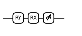
电路可视化。

from isqtools.draw import Drawer

dr = Drawer()
dr.plot(qc1.qcis)

2. 使用Pytorch进行自动微分

和轻量级自动求导工具Autograd相比，Pytorch是一个高效的机器学习框架。Pytorch可以充分调动CPU、GPU资源，计算效率更高。我们非常建议学习一下Pytorch的基础教程以及自动求导教程。

import torch 


torch_backend = TorchBackend()

qc2 = IsqCircuit(
    file="gradient.isq",
    backend=torch_backend,
    sample=False,
)

params2 = torch.tensor([0.9, 1.2], requires_grad=True)

def circuit2(params2):
    return qc2.measure(params=params2)[0]

result = circuit2(params2)
result.backward()

print(result)
print(params2.grad)

tensor(0.6126, grad_fn=<SelectBackward0>)
tensor([-0.1419, -0.2897])

电路可视化。

from isqtools.draw import Drawer

dr = Drawer()
dr.plot(qc2.qcis)