python模拟器

除了使用isqc自带的模拟器之外，我们还额外提供了基于python的模拟器。

1. 创建isQ代码

这段代码命名为python_sim_quick_start.isq，并且放在同一个目录。
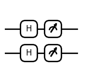
该文件创建了2个量子比特，分别使用H门作用这两个比特，最后测量。

import std;


qbit q[2];

unit main() {
    H(q[0]);
    H(q[1]);
    M(q[0]);
    M(q[1]);
}

2. 创建量子电路

我们提供了IsqCircuit进行创建量子线路，NumpyBackend, AutogradBackend, TorchBackend三种不同的模拟后台。

from isqtools import IsqCircuit
from isqtools.backend import NumpyBackend, AutogradBackend, TorchBackend

首先，我们使用最基础的NumPy作为模拟后台，对该电路进行模拟。

backend = NumpyBackend()
qc = IsqCircuit(
    file="python_sim_quick_start.isq",
    backend=backend,
    sample=False,
)

print(f"Probability results:", qc.measure())
print("Each item of the array represents these states:"
      ,"`00`", "`01`", "`10`", "`11`")
print()
print(f"Qcis:\n{qc}")

Probability results: [0.25 0.25 0.25 0.25]
Each item of the array represents these states: `00` `01` `10` `11`

Qcis:
H Q0
H Q1
M Q0
M Q1

我们建立了IsqCircuit的实例qc，建立时传入的backend参数代表模拟器的后台，sample参数表示是否使用采样模式。对于是否使用采样模式，教程下方有详细的实例演示。

qc.measure()对该电路进行测量，该电路我们未进行采样，没有shots的概念，此时输出的是该量子电路测量的理论概率分布。对于2个qubit的情况，有4中可能的输出状态，分别是00 01 10 11，我们测量的返回结果分别代表这4种状态的理论概率分布。

我们可以使用print(qc)打印isq文件编译生成Qcis指令集。

3. 非采样模式

当采样sample=False时候，三种后台NumpyBackend, AutogradBackend, TorchBackend都输出对应的概率分布。注意当使用pytorch作为后台时，输出的结果类型为torch.Tensor。

backends = {
    "numpy": NumpyBackend(),
    "autograd": AutogradBackend(),
    "torch": TorchBackend(),
}

for backend_name, backend in backends.items():
    qc = IsqCircuit(
        file="python_sim_quick_start.isq",
        backend=backend,
        sample=False,
    )
    print(f"Probability results of {backend_name}: {qc.measure()}, "
          f"and return type: {type(qc.measure())}")

Probability results of numpy: [0.25 0.25 0.25 0.25], and return type: <class 'numpy.ndarray'>
Probability results of autograd: [0.25 0.25 0.25 0.25], and return type: <class 'numpy.ndarray'>
Probability results of torch: tensor([0.2500, 0.2500, 0.2500, 0.2500]), and return type: <class 'torch.Tensor'>

4. 采样模式

当采样sample=True时候，三种后台NumpyBackend, AutogradBackend, TorchBackend都输出对应的采样结果，此时需要指定shots的数值，默认shots为100。注意此时输出的结果类型为python内置的dict。这里的dict并不保证量子比特的顺序，10可能出现在00前面。

for backend_name, backend in backends.items():
    qc = IsqCircuit(
        file="python_sim_quick_start.isq",
        backend=backend,
        sample=True,
        shots=1000,
    )
    print(f"Sample results of {backend_name}: {qc.measure()}, "
          f"and return type: {type(qc.measure())}")

Sample results of numpy: {'11': 253, '10': 256, '01': 239, '00': 252}, and return type: <class 'dict'>
Sample results of autograd: {'10': 240, '00': 269, '01': 236, '11': 255}, and return type: <class 'dict'>
Sample results of torch: {'01': 237, '00': 242, '10': 270, '11': 251}, and return type: <class 'dict'>

如果对测量结果的顺序比较关系，可以使用以下的方法进行转换。

res_dict = qc.measure()
ordered_res_dict = qc.sort_dict(res_dict)
res_dict_array = qc.dict2array(res_dict)
print(f"Naive sample results {res_dict}.")
print(f"Ordered Sample results {ordered_res_dict}.")
print(f"Transfer Sample results to array: {res_dict_array}.")

Naive sample results {'11': 222, '10': 276, '00': 259, '01': 243}.
Ordered Sample results {'00': 259, '01': 243, '10': 276, '11': 222}.
Transfer Sample results to array: [0.259 0.243 0.276 0.222].

5. 电路可视化

对于isq文件生成的Qcis指令集，我们提供了简单的画图接口。

from isqtools.draw import Drawer

backend = NumpyBackend()
qc = IsqCircuit(
    file="python_sim_quick_start.isq",
    backend=backend,
    sample=False,
)

dr = Drawer()
dr.plot(qc.qcis)