Quantum Machine Learning Basics
Using the PyTorch Backend Simulator
The isq simulator uses PyTorch as its backend, making it easy to simulate quantum machine learning tasks.
First, import the necessary packages. To ensure the reproducibility of the experiment, we fix the random seed.
[1]:
import random

import numpy as np
import torch
import torch.optim as optim

from isqtools import IsqCircuit
from isqtools.backend import TorchBackend
from isqtools.neural_networks import TorchLayer


def setup_seed(seed):
    torch.manual_seed(seed)
    torch.cuda.manual_seed_all(seed)
    np.random.seed(seed)
    random.seed(seed)


setup_seed(222)
Define param Variables for Automatic Differentiation
For quantum machine learning tasks, we need to define arrays of parameterized variables in the .isq file using the syntax param inputs[]; and param weights[];. We recommend defining two such variables. If more parameter arrays are required, you may need to implement the gradient computation logic yourself in the TorchLayer or TorchWrapper.
Currently, the param variables defined in isq support three types of rotation gates: RX, RY, and RZ.
Refer to the .isq file below for the specific definition. The file is named nn_basic.isq.
import std;


param inputs[], weights[];
qbit q[4];
int pauli_inx[] = [2, 2, 3, 3]; // this means Z0Z1I2I3

// using arrays for pauli measurement,
// X:0, Y:1, Z:2, I:3

procedure single_h(qbit q[]) {
    for i in 0:q.length {
        H(q[i]);
    }
}

procedure adjacent_cz(qbit q[]) {
    for i in 0:q.length-1 {
        CZ(q[i], q[i+1]);
    }
}

procedure encode_inputs(qbit q[], int start_idx) {
    for i in 0:q.length {
        Rz(inputs[i+start_idx], q[i]);
    }
}

procedure encode_weights(qbit q[], int start_idx) {
    for i in 0:q.length {
        Ry(weights[i+start_idx], q[i]);
    }
    for i in 0:q.length {
        Rx(weights[i+start_idx+4], q[i]);
    }
}

procedure pauli(int pauli_idx[], qbit q[]) {
    assert pauli_idx.length == q.length;
    for i in 0:q.length {
        if (pauli_idx[i] == 0) {
            H(q[i]);
            M(q[i]);
        }
        if (pauli_idx[i] == 1) {
            X2P(q[i]);
            M(q[i]);
        }
        if (pauli_idx[i] == 2) {
            M(q[i]);
        }
        if (pauli_idx[i] == 3) {
            continue;
        }
    }
}

procedure main() {

    single_h(q);
    encode_inputs(q, 0);
    adjacent_cz(q);

    encode_weights(q, 0);
    adjacent_cz(q);

    encode_weights(q, 8);
    adjacent_cz(q);

    encode_weights(q, 16);
    adjacent_cz(q);

    pauli(pauli_inx, q);
}
We use tempfileto simulate here.
[2]:
FILE_CONTENT = """\
import std;


param inputs[], weights[];
qbit q[4];
int pauli_inx[] = [2, 2, 3, 3]; // this means Z0Z1I2I3

// using arrays for pauli measurement,
// X:0, Y:1, Z:2, I:3

procedure single_h(qbit q[]) {
    for i in 0:q.length {
        H(q[i]);
    }
}

procedure adjacent_cz(qbit q[]) {
    for i in 0:q.length-1 {
        CZ(q[i], q[i+1]);
    }
}

procedure encode_inputs(qbit q[], int start_idx) {
    for i in 0:q.length {
        Rz(inputs[i+start_idx], q[i]);
    }
}

procedure encode_weights(qbit q[], int start_idx) {
    for i in 0:q.length {
        Ry(weights[i+start_idx], q[i]);
    }
    for i in 0:q.length {
        Rx(weights[i+start_idx+4], q[i]);
    }
}

procedure pauli(int pauli_idx[], qbit q[]) {
    assert pauli_idx.length == q.length;
    for i in 0:q.length {
        if (pauli_idx[i] == 0) {
            H(q[i]);
            M(q[i]);
        }
        if (pauli_idx[i] == 1) {
            X2P(q[i]);
            M(q[i]);
        }
        if (pauli_idx[i] == 2) {
            M(q[i]);
        }
        if (pauli_idx[i] == 3) {
            continue;
        }
    }
}

procedure main() {

    single_h(q);
    encode_inputs(q, 0);
    adjacent_cz(q);

    encode_weights(q, 0);
    adjacent_cz(q);

    encode_weights(q, 8);
    adjacent_cz(q);

    encode_weights(q, 16);
    adjacent_cz(q);

    pauli(pauli_inx, q);
}"""
For quantum machine learning simulation tasks, we highly recommend using PyTorch as the simulation backend. PyTorch supports automatic differentiation, making it easy to compute the gradients of parameterized circuits. It also supports parallelism and GPU acceleration, offering high computational efficiency. Additionally, with torch.vmap (available in PyTorch version 2.0 and above), you can efficiently perform batched circuit simulations, which is significantly faster than using a simple
for-loop.
[3]:
import tempfile
from pathlib import Path
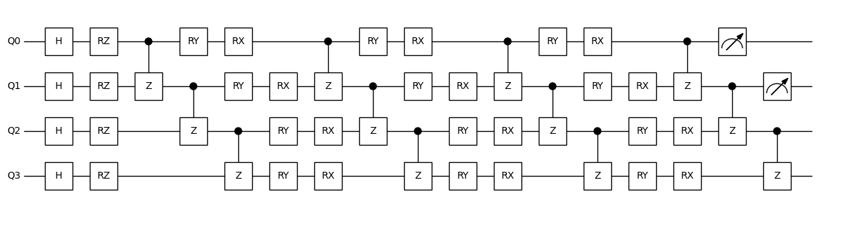
from isqtools.draw import Drawer
backend = TorchBackend()
with tempfile.TemporaryDirectory() as temp_dir:
temp_dir_path = Path(temp_dir)
temp_file_path = temp_dir_path / "nn_basic.isq"
with open(temp_file_path, "w") as temp_file:
temp_file.write(FILE_CONTENT)
qc = IsqCircuit(
file=temp_file_path,
backend=backend,
sample=False,
)
dr = Drawer()
dr.plot(qc.qcis)
Create a Quantum Circuit
To build a quantum circuit for quantum machine learning, we first need to define a function. Below is an example using a function named circuit.
This function takes two arguments: inputs and weights. Here, inputs represents the data to be encoded. The circuit simulation and measurement are performed using the pauli_measure() method. When using pauli_measure(), a basis transformation must be implemented in the .isq file. We have provided an example of this in nn_basic.isq with the procedure procedure pauli(int pauli_idx[], qbit q[]).
Advanced users may define custom measurement procedures if needed. When using parameterized circuits, parameters should be passed in key-value form. The syntax **param unpacks a Python dictionary, which is equivalent to passing arguments in key-value pairs. Each key should match the parameter names defined in the .isq file (e.g., param inputs[], param weights[] in nn_basic.isq), and each value corresponds to the input arguments of the Python function
def circuit(inputs, weights).
[4]:
def circuit(inputs, weights):

    param = {
        "inputs": inputs,
        "weights": weights,
    }

    return qc.pauli_measure(**param)
Forward Measurement Circuit
When using PyTorch as the simulation backend, we define the parameters as torch.Tensor objects.
In this example, we randomly generate inputs and weights, then pass them to the circuit function. This will return the result of the Pauli measurement.
[5]:
inputs = torch.randn(4)
weights = torch.randn(24)
weights_backup = weights.clone()
inputs_backup = inputs.clone()
print(f"{inputs=}")
print(f"{weights=}")
print("Result:", circuit(inputs, weights))
inputs=tensor([-0.4248,  1.1523, -2.1342,  0.5376])
weights=tensor([ 0.3889, -0.7956, -0.4133, -0.2245, -1.3118,  0.4663, -0.9789,  1.3999,
         1.6718,  0.1663, -0.4762, -1.0917,  0.5813, -0.1228, -0.0768, -0.7945,
        -0.8038, -0.1344, -0.9184, -0.3778,  0.4568,  0.7652,  0.4885, -2.1489])
Result: tensor(-0.1275)
Create a Quantum Machine Learning Layer
By using TorchLayer and passing in the previously defined circuit function along with some necessary parameters, we can obtain a qnn object that inherits from torch.nn.Module.
is_vmap=False indicates that vmap is not used.
num_weights specifies the length of the weights parameter.
initial_weights allows you to provide a custom initialization for the weights; if not specified, the parameters will be initialized automatically.
We can compare the outputs of circuit and qnn to observe the difference. Pay attention to how the parameters are passed. Thanks to the use of torch.nn.Module, gradient information is automatically constructed for the qnn layer.
[6]:
qnn = TorchLayer(
    circuit=circuit,
    is_vmap=False,
    num_weights=24,
    initial_weights=weights,
)

print(qnn)
print(qnn.__class__.__bases__)
print()
print("Run circuit:", circuit(inputs, weights))
print("Run qnn:", qnn(inputs))
TorchLayer(num_weights=24, is_vmap=False)
(<class 'torch.nn.modules.module.Module'>,)

Run circuit: tensor(-0.1275)
Run qnn: tensor(-0.1275, grad_fn=<DotBackward0>)
Optimize the Quantum Circuit
Since qnn inherits from torch.nn.Module, we can conveniently use PyTorch’s optimizers to optimize it.
In this example, we apply SGD (Stochastic Gradient Descent) to update the weights while keeping inputs fixed, aiming to minimize the output of qnn, which corresponds to the result of the Pauli measurement.
After 50 optimization steps, the Pauli measurement value converges to its minimum, which is -1.
[7]:
optimizer = optim.SGD(qnn.parameters(), lr=0.05)

for i in range(50):
    measurement = qnn(inputs)
    measurement.backward()
    optimizer.step()
    optimizer.zero_grad()
    if i % 5 == 0:
        print(measurement)
tensor(-0.1275, grad_fn=<DotBackward0>)
tensor(-0.3230, grad_fn=<DotBackward0>)
tensor(-0.4942, grad_fn=<DotBackward0>)
tensor(-0.6281, grad_fn=<DotBackward0>)
tensor(-0.7245, grad_fn=<DotBackward0>)
tensor(-0.7911, grad_fn=<DotBackward0>)
tensor(-0.8372, grad_fn=<DotBackward0>)
tensor(-0.8697, grad_fn=<DotBackward0>)
tensor(-0.8935, grad_fn=<DotBackward0>)
tensor(-0.9115, grad_fn=<DotBackward0>)
You can print the optimized inputs and weights after the training process.
As inputs serve as the fixed input data, they remain unchanged throughout the optimization. In contrast, weights are gradually updated and optimized toward their optimal values, causing the Pauli measurement output to approach -1.
[8]:
print(f"{inputs}")
print(f"{inputs_backup}")
print("Optimized weights:", weights)
print(f"{weights_backup=}")
tensor([-0.4248,  1.1523, -2.1342,  0.5376])
tensor([-0.4248,  1.1523, -2.1342,  0.5376])
Optimized weights: tensor([ 0.3963, -0.4383, -0.5218, -0.2149, -1.5535,  1.0736, -0.9547,  1.4377,
         2.3391, -0.0104, -0.1606, -1.0917,  0.4081, -0.2264, -0.2291, -0.7945,
        -1.0293, -0.6749, -0.9184, -0.3778,  0.4045,  0.9554,  0.4885, -2.1489])
weights_backup=tensor([ 0.3889, -0.7956, -0.4133, -0.2245, -1.3118,  0.4663, -0.9789,  1.3999,
         1.6718,  0.1663, -0.4762, -1.0917,  0.5813, -0.1228, -0.0768, -0.7945,
        -0.8038, -0.1344, -0.9184, -0.3778,  0.4568,  0.7652,  0.4885, -2.1489])
Environment Information
The following versions of software and libraries are used in this tutorial:
[9]:
import platform
import subprocess
from importlib.metadata import version

print(f"Python version used in this tutorial: {platform.python_version()}")
print(f"Execution environment: {platform.system()} {platform.release()}\n")


isqc_version = subprocess.check_output(
    ["isqc", "-V"], stderr=subprocess.STDOUT, text=True
).strip()
print(f"isqc version: {isqc_version}")

isqtools_version = version("isqtools")
print(f"isqtools version: {isqtools_version}")

numpy_version = version("numpy")
print(f"NumPy version: {numpy_version}")

torch_version = version("torch")
print(f"Torch version: {torch_version}")
Python version used in this tutorial: 3.13.5
Execution environment: Linux 6.12.45

isqc version: isQ Compiler 0.2.5
isqtools version: 1.4.1
NumPy version: 2.3.1
Torch version: 2.7.1