Python Simulator

In addition to the built-in simulator provided by isqc, we also provide an additional simulator based on Python.

Create isQ Code

Name the code file python_sim_quick_start.isq and place it in the same directory.

This file creates two qubits, applies an H gate to each of them, and performs measurement at the end.

import std;


qbit q[2];

unit main() {
    H(q[0]);
    H(q[1]);
    M(q[0]);
    M(q[1]);
}

We use tempfile instead of a real file.

FILE_CONTENT = """\
import std;


qbit q[2];

unit main() {
    H(q[0]);
    H(q[1]);
    M(q[0]);
    M(q[1]);
}"""

Create Quantum Circuit

We provide IsqCircuit for building quantum circuits, along with three different simulation backends: NumpyBackend, AutogradBackend, and TorchBackend.

First, we use the basic NumPy backend to simulate the circuit.

import tempfile
from pathlib import Path

from isqtools import IsqCircuit
from isqtools.backend import AutogradBackend, NumpyBackend, TorchBackend

with tempfile.TemporaryDirectory() as temp_dir:
    temp_dir_path = Path(temp_dir)
    temp_file_path = temp_dir_path / "python_sim_quick_start.isq"
    with open(temp_file_path, "w") as temp_file:
        temp_file.write(FILE_CONTENT)

    backend = NumpyBackend()
    qc = IsqCircuit(
        file=str(temp_file_path),
        backend=backend,
        sample=False,
    )

    print(f"Probability results:", qc.measure())
    print(
        "Each item of the array represents these states:",
        "`00`",
        "`01`",
        "`10`",
        "`11`",
    )
    print()
    print(f"Qcis:\n{qc}")

Probability results: [0.25 0.25 0.25 0.25]
Each item of the array represents these states: `00` `01` `10` `11`

Qcis:
H Q0
H Q1
M Q0
M Q1

Non-Sampling Mode

When sample=False, all three backends—NumpyBackend, AutogradBackend, and TorchBackend—output the corresponding probability distribution.

Note that when using PyTorch as the backend, the output type is torch.Tensor.

with tempfile.TemporaryDirectory() as temp_dir:
    temp_dir_path = Path(temp_dir)
    temp_file_path = temp_dir_path / "python_sim_quick_start.isq"
    with open(temp_file_path, "w") as temp_file:
        temp_file.write(FILE_CONTENT)

    backends = {
        "numpy": NumpyBackend(),
        "autograd": AutogradBackend(),
        "torch": TorchBackend(),
    }

    for backend_name, backend in backends.items():
        qc = IsqCircuit(
            file=str(temp_file_path),
            backend=backend,
            sample=False,
        )
        print(
            f"Probability results of {backend_name}: {qc.measure()}, "
            f"and return type: {type(qc.measure())}"
        )

Probability results of numpy: [0.25 0.25 0.25 0.25], and return type: <class 'numpy.ndarray'>
Probability results of autograd: [0.25 0.25 0.25 0.25], and return type: <class 'numpy.ndarray'>
Probability results of torch: tensor([0.2500, 0.2500, 0.2500, 0.2500]), and return type: <class 'torch.Tensor'>

Sampling Mode

When sample=True, all three backends—NumpyBackend, AutogradBackend, and TorchBackend—output the corresponding sampling results. In this mode, you need to specify the number of shots; by default, shots=100.

Note that the output is a Python built-in dict, and the order of qubit outcomes is not guaranteed—e.g., 10 may appear before 00.

with tempfile.TemporaryDirectory() as temp_dir:
    temp_dir_path = Path(temp_dir)
    temp_file_path = temp_dir_path / "python_sim_quick_start.isq"
    with open(temp_file_path, "w") as temp_file:
        temp_file.write(FILE_CONTENT)
    for backend_name, backend in backends.items():
        qc = IsqCircuit(
            file=str(temp_file_path),
            backend=backend,
            sample=True,
            shots=1000,
        )
        print(
            f"Sample results of {backend_name}: {qc.measure()}, "
            f"and return type: {type(qc.measure())}"
        )

Sample results of numpy: {'11': 260, '00': 241, '10': 242, '01': 257}, and return type: <class 'dict'>
Sample results of autograd: {'00': 229, '01': 262, '10': 270, '11': 239}, and return type: <class 'dict'>
Sample results of torch: {'10': 277, '11': 238, '00': 236, '01': 249}, and return type: <class 'dict'>

If you need to compare the order of measurement results, you can convert them using the following method.

res_dict = qc.measure()
ordered_res_dict = qc.sort_dict(res_dict)
res_dict_array = qc.dict2array(res_dict)
print(f"Naive sample results {res_dict}.")
print(f"Ordered Sample results {ordered_res_dict}.")
print(f"Transfer Sample results to array: {res_dict_array}.")

Naive sample results {'11': 279, '01': 237, '10': 238, '00': 246}.
Ordered Sample results {'00': 246, '01': 237, '10': 238, '11': 279}.
Transfer Sample results to array: [0.246 0.237 0.238 0.279].

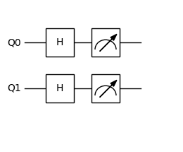
Circuit Visualization

For the QCIS instruction set generated from isQ files, we provide a simple interface for circuit visualization.

from isqtools.draw import Drawer

with tempfile.TemporaryDirectory() as temp_dir:
    temp_dir_path = Path(temp_dir)
    temp_file_path = temp_dir_path / "python_sim_quick_start.isq"
    with open(temp_file_path, "w") as temp_file:
        temp_file.write(FILE_CONTENT)
    backend = NumpyBackend()
    qc = IsqCircuit(
        file=str(temp_file_path),
        backend=backend,
        sample=False,
    )

    dr = Drawer()
    dr.plot(qc.qcis)

Environment Information

The following versions of software and libraries are used in this tutorial:

import platform
import subprocess
from importlib.metadata import version

print(f"Python version used in this tutorial: {platform.python_version()}")
print(f"Execution environment: {platform.system()} {platform.release()}\n")


isqc_version = subprocess.check_output(
    ["isqc", "-V"], stderr=subprocess.STDOUT, text=True
).strip()
print(f"isqc version: {isqc_version}")

isqtools_version = version("isqtools")
print(f"isqtools version: {isqtools_version}")

numpy_version = version("numpy")
print(f"NumPy version: {isqtools_version}")

autograd_version = version("autograd")
print(f"Autograd version: {autograd_version}")

torch_version = version("torch")
print(f"Torch version: {torch_version}")

Python version used in this tutorial: 3.13.5
Execution environment: Linux 6.12.41

isqc version: isQ Compiler 0.2.5
isqtools version: 1.3.0
NumPy version: 1.3.0
Autograd version: 1.8.0
Torch version: 2.7.1