Variational quantum eigensolver
The eigenvalues of the Hamiltonian determine almost all properties in a molecule or material of interest. The ground state for molecule Hamiltonian is of particular interest since the energy gap between the ground state and the first excited state of electrons at room temperature is usually larger. Most molecules are in the ground state.
Here, molecular electronic Hamiltonian is represented as \(\hat{H}\). A trial wave function \(|\varphi(\theta)\rangle\) is parameterized with \(\vec{\theta}\), which is called Ansatz. VQE is represented as follows:
\(E_0\) is the lowest energy of the molecular electronic Hamiltonian \(\hat{H}\). To estimate \(E_0\), the left-hand side of the equation above is minimized by updating the parameters of the Ansatz \(|\varphi(\theta)\rangle\).
The molecular electronic Hamiltonian \(\hat{H}\) has the second quantized form:
It can be mapped to the linear combination of Pauli operator by Jordan-Wigner transformation or Bravyi-Kitaev transformation as follows:
Then, we calculate the expectation value of the Hamiltonian \(\hat{H}\) with respect to the Ansatz \(|\varphi(\theta)\rangle\) by designing a quantum circuit. Finally, we update the parameters in the Ansatz circuit to minimize the energy and obtain \(E_0\), the lowest energy of the molecular electronic Hamiltonian.
The overview of VQE schematic diagram is as follows:
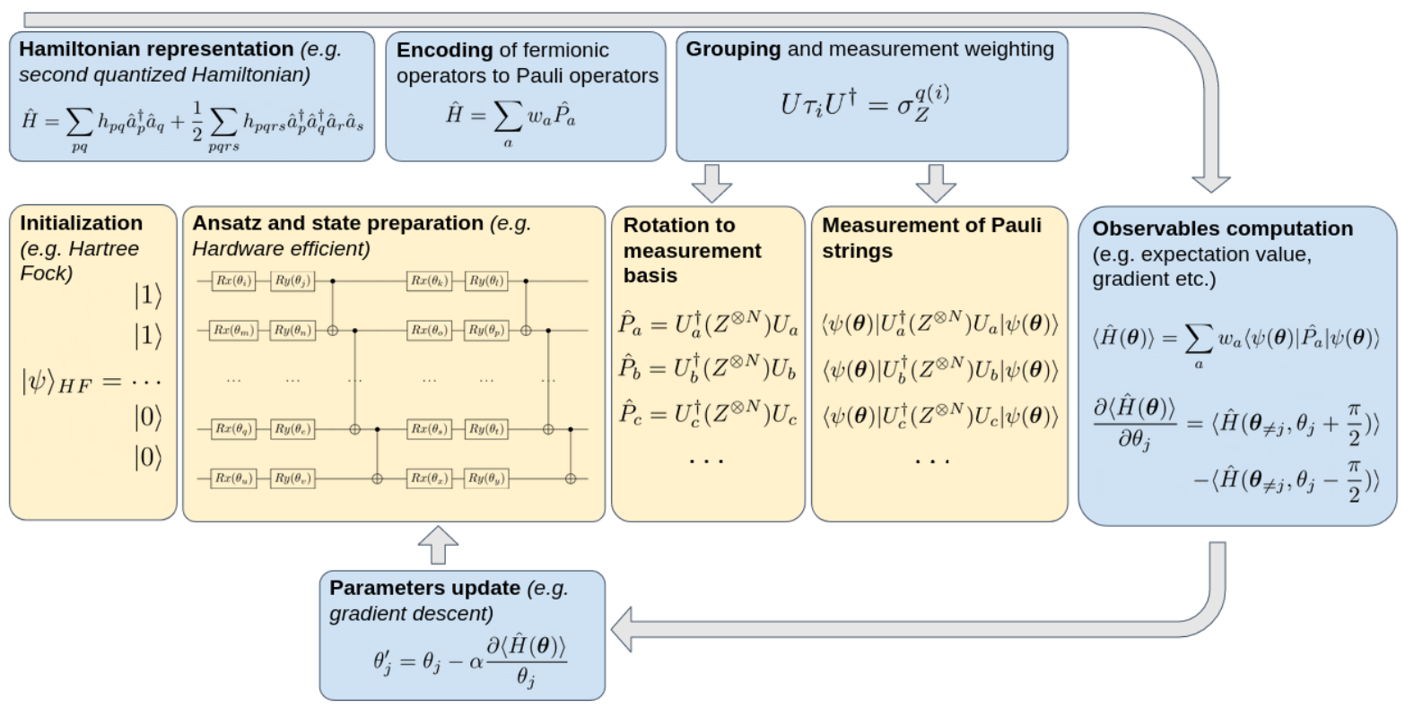
VQE belongs to the class of hybrid quantum-classical algorithms, in which the quantum computer is responsible for executing quantum circuits, while the classical computer updates the parameters of quantum gates in the Ansatz \(|\varphi(\theta)\rangle\).
Through this process, the lowest energy of the molecular electronic Hamiltonian \(\hat{H}\), denoted as \(E_0\), can be obtained, along with the corresponding wave function.
To illustrate the algorithm flow, we take the estimation of the ground-state energy of the hydrogen molecule as an example. After applying the Jordan–Wigner transformation in a minimal basis, the Hamiltonian becomes:
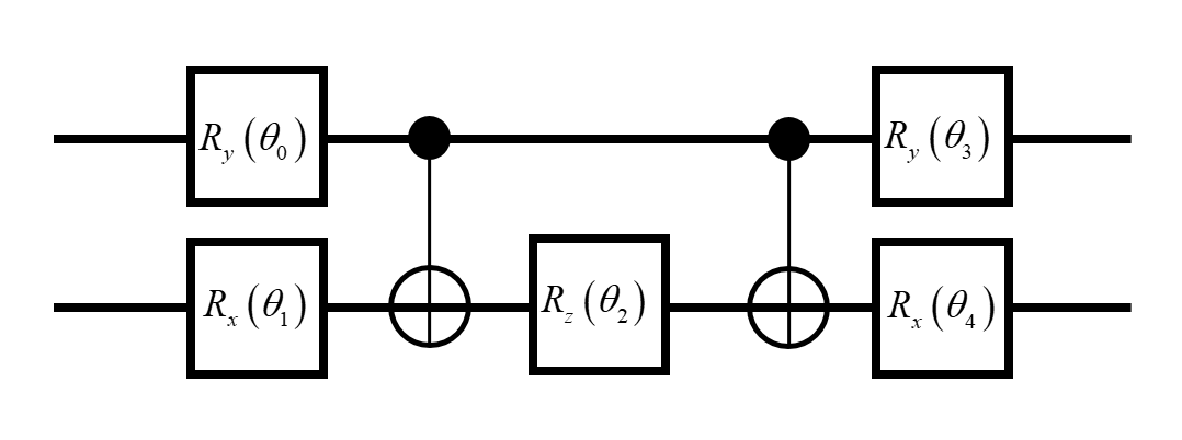
We use two qubits in this example. The Ansatz \(|\varphi(\theta)\rangle\) is:
H2 Hamiltonian.[6]:
coeffs = [-0.4804, +0.3435, -0.4347, +0.5716, +0.0910, +0.0910]
gates_group = [
    ((0, "Z"),),
    ((1, "Z"),),
    ((0, "Z"), (1, "Z")),
    ((0, "Y"), (1, "Y")),
    ((0, "X"), (1, "X")),
]
We use tempfile to run h2.isq. We use isqtools to compile isq file.
[7]:
H2_FILE_CONTENT = """\
import std;

int num_qubits = 2;
int pauli_gates[] = [
    3, 0,
    0, 3,
    3, 3,
    2, 2,
    1, 1
];
// Hamiltonian gates: Z0, Z1, Z0Z1, Y0Y1, X0X2
unit vqe_measure(qbit q[], int idx) {
    // using arrays for pauli measurement
    // I:0, X:1, Y:2, Z:3
    int start_idx = num_qubits*idx;
    int end_idx = num_qubits*(idx+1);

    for i in start_idx:end_idx {
        if (pauli_gates[i] == 0) {
            // I:0
            continue;
        }
        if (pauli_gates[i] == 1) {
            // X:1
            H(q[i%num_qubits]);
            M(q[i%num_qubits]);
        }
        if (pauli_gates[i] == 2) {
            // Y:2
            X2P(q[i%num_qubits]);
            M(q[i%num_qubits]);
        }
        if (pauli_gates[i] == 3) {
            // Z:3
            M(q[i%num_qubits]);
        }
    }
}

unit main(int i_par[], double d_par[]) {

    qbit q[2];
    X(q[1]);

    Ry(1.57, q[0]);
    Rx(4.71, q[1]);
    CNOT(q[0],q[1]);
    Rz(d_par[0], q[1]);
    CNOT(q[0],q[1]);
    Ry(4.71, q[0]);
    Rx(1.57, q[1]);

    vqe_measure(q, i_par[0]);
}
"""
[8]:
import tempfile
import time
from pathlib import Path

import numpy as np

from isqtools.utils import isqc_compile, isqc_simulate

shots = 100
learning_rate = 1.0
energy_list = []
epochs = 20
theta = np.array([0.0])


def get_expectation(theta):
    measure_results = np.zeros(len(gates_group) + 1)
    measure_results[0] = 1.0
    # The first does not require quantum measurement, which is constant
    # As a result, the other 5 coefficients need to be measured
    for idx in range(len(gates_group)):
        result_dict = isqc_simulate(
            temp_dir_path / "h2.so",
            shots=shots,
            int_param=idx,
            double_param=theta,
        )[0]
        result = 0
        for res_index, frequency in result_dict.items():
            parity = (-1) ** (res_index.count("1") % 2)
            # parity checking to get expectation value
            result += parity * frequency / shots
            # frequency instead of probability
        measure_results[idx + 1] = result
        # to accumulate every expectation result
        # The result is multiplied by coefficient
    return np.dot(measure_results, coeffs)


def parameter_shift(theta):
    # to get gradients
    theta = theta.copy()
    theta += np.pi / 2
    forwards = get_expectation(theta)
    theta -= np.pi
    backwards = get_expectation(theta)
    return 0.5 * (forwards - backwards)


with tempfile.TemporaryDirectory() as temp_dir:
    temp_dir_path = Path(temp_dir)
    temp_file_path = temp_dir_path / "h2.isq"
    with open(temp_file_path, "w") as temp_file:
        temp_file.write(H2_FILE_CONTENT)
    isqc_compile(file=temp_file_path, target="qir")
    # compile "h2.isq" and generate the qir file "h2.so"
    energy = get_expectation(theta)
    energy_list.append(energy)
    print(f"Initial VQE Energy: {energy_list[0]} Hartree")
    start_time = time.time()
    for epoch in range(epochs):
        theta -= learning_rate * parameter_shift(theta)
        energy = get_expectation(theta)
        energy_list.append(energy)
        print(f"Epoch {epoch+1}: {energy} Hartree")

    print(f"Final VQE Energy: {energy_list[-1]} Hartree")
    print("Time:", time.time() - start_time)
Initial VQE Energy: -0.27562 Hartree
Epoch 1: -0.35547 Hartree
Epoch 2: -0.4695019999999999 Hartree
Epoch 3: -0.827114 Hartree
Epoch 4: -1.5788099999999998 Hartree
Epoch 5: -1.856718 Hartree
Epoch 6: -1.841756 Hartree
Epoch 7: -1.85386 Hartree
Epoch 8: -1.835468 Hartree
Epoch 9: -1.8364760000000002 Hartree
Epoch 10: -1.86114 Hartree
Epoch 11: -1.8710600000000002 Hartree
Epoch 12: -1.87024 Hartree
Epoch 13: -1.871462 Hartree
Epoch 14: -1.869638 Hartree
Epoch 15: -1.8281880000000001 Hartree
Epoch 16: -1.8633660000000003 Hartree
Epoch 17: -1.8506260000000003 Hartree
Epoch 18: -1.856492 Hartree
Epoch 19: -1.8419400000000004 Hartree
Epoch 20: -1.8318280000000002 Hartree
Final VQE Energy: -1.8318280000000002 Hartree
Time: 6.900815486907959
Environment Information
The following versions of software and libraries are used in this tutorial:
[9]:
import platform
import subprocess
from importlib.metadata import version

print(f"Python version used in this tutorial: {platform.python_version()}")
print(f"Execution environment: {platform.system()} {platform.release()}\n")


isqc_version = subprocess.check_output(
    ["isqc", "-V"], stderr=subprocess.STDOUT, text=True
).strip()
print(f"isqc version: {isqc_version}")

isqtools_version = version("isqtools")
print(f"isqtools version: {isqtools_version}")

numpy_version = version("numpy")
print(f"NumPy version: {numpy_version}")
Python version used in this tutorial: 3.13.5
Execution environment: Linux 6.12.45

isqc version: isQ Compiler 0.2.5
isqtools version: 1.4.1
NumPy version: 2.3.1
Reference
Tilly, H. Chen, S. Cao, et al. “The variational quantum eigensolver: a review of methods and best practices.” Physics Reports, 2022, 986: 1-128.
O’Malley et al. “Scalable Quantum Simulation of Molecular Energies.” Physics Review X, 6, 031007, 2016.