Autograd

Creating isQ Code

In general quantum circuit simulations, we recommend using sample=False. This simulation method yields exact measurement results of the quantum circuit (i.e., theoretical probability distributions), without concerns about the number of shots. The exact simulation result corresponds to the limit as the number of shots approaches infinity.

When using exact simulation, another benefit is the ability to compute gradients of parameters analytically by using the AutogradBackend or TorchBackend. First, we construct a quantum circuit that contains parameters params[].

This piece of code should be named gradient.isq and placed in the same directory.

import std;


param params[];
qbit q[1];

unit main() {
    Ry(params[0], q[0]);
    Rx(params[1], q[0]);
    M(q[0]);
}

We use tempfileto simulate here.

FILE_CONTENT = """\
import std;


param params[];
qbit q[1];

unit main() {
    Ry(params[0], q[0]);
    Rx(params[1], q[0]);
    M(q[0]);
}"""

Automatic Differentiation with Autograd

Autograd, a lightweight extension of NumPy, can be used to perform automatic differentiation. First, we use AutogradBackend as the simulation backend and set sample=False to obtain exact simulation results. Then, we define a NumPy array params1 and a function circuit1.

Within the function, we call qc1.measure(params=params1), passing our parameters as a keyword argument. Here, the left side of params=params1 corresponds to the parameter definition in gradient.isq, while the right side refers to the params1array defined in Python. The return value of the function circuit1 is the first element of the measurement result array, i.e., results[0].

import tempfile
from pathlib import Path

import numpy as np
from isqtools import IsqCircuit
from isqtools.backend import AutogradBackend, TorchBackend

with tempfile.TemporaryDirectory() as temp_dir:
    temp_dir_path = Path(temp_dir)
    temp_file_path = temp_dir_path / "gradient.isq"
    with open(temp_file_path, "w") as temp_file:
        temp_file.write(FILE_CONTENT)

    autograd_backend = AutogradBackend()

    qc1 = IsqCircuit(
        file=str(temp_file_path),
        backend=autograd_backend,
        sample=False,
    )

    params1 = np.array([0.9, 1.2])

    def circuit1(params1):
        results = qc1.measure(params=params1)
        return results[0]

    print(circuit1(params1))

0.6126225961314372

At this point, we can use the grad function from Autograd to compute the derivative of the circuit1 function. The grad function accepts the index of the parameter to differentiate with respect to as its second argument. In this case, since circuit1 has only one parameter params1, we can pass [0] as the index for differentiation.

The grad function returns a callable object, which takes the same input as the original function and returns the gradient with respect to the specified parameter. For more advanced usage, please refer to the official Autograd documentation.

from autograd import grad


params1 = np.array([0.9, 1.2])

def circuit1(params1):
    results = qc1.measure(params=params1)
    return results[0]

grad_circuit1 = grad(circuit1, [0])
print(grad_circuit1(params1))

(array([-0.14192229, -0.28968239]),)

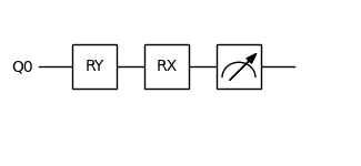
Circuit Visualization

We provide a simple interface for visualizing quantum circuits generated from .qcis files. Once you have written your quantum circuit, you can use the built-in visualization tools to render the circuit diagram. This helps in understanding the structure and flow of the quantum gates applied in the circuit.

The visualization interface supports basic gates and parameterized gates, and is especially useful for debugging and presentation purposes.

from isqtools.draw import Drawer


dr = Drawer()
dr.plot(qc1.qcis)

Automatic Differentiation with PyTorch

Compared to the lightweight Autograd library, PyTorch is a powerful and efficient machine learning framework. PyTorch can fully utilize CPU and GPU resources, offering significantly higher computational efficiency.

We highly recommend exploring PyTorch’s basic tutorials as well as its automatic differentiation tutorials to get familiar with its functionality and gradient computation capabilities.

import torch

with tempfile.TemporaryDirectory() as temp_dir:
    temp_dir_path = Path(temp_dir)
    temp_file_path = temp_dir_path / "gradient.isq"
    with open(temp_file_path, "w") as temp_file:
        temp_file.write(FILE_CONTENT)
    torch_backend = TorchBackend()

    qc2 = IsqCircuit(
        file=str(temp_file_path),
        backend=torch_backend,
        sample=False,
    )

    params2 = torch.tensor([0.9, 1.2], requires_grad=True)

    def circuit2(params2):
        return qc2.measure(params=params2)[0]

    result = circuit2(params2)
    result.backward()

    print(result)
    print(params2.grad)
    dr = Drawer()
    dr.plot(qc2.qcis)

tensor(0.6126, grad_fn=<SelectBackward0>)
tensor([-0.1419, -0.2897])

Environment Information

The following versions of software and libraries are used in this tutorial:

import platform
import subprocess
from importlib.metadata import version

print(f"Python version used in this tutorial: {platform.python_version()}")
print(f"Execution environment: {platform.system()} {platform.release()}\n")


isqc_version = subprocess.check_output(
    ["isqc", "-V"], stderr=subprocess.STDOUT, text=True
).strip()
print(f"isqc version: {isqc_version}")

isqtools_version = version("isqtools")
print(f"isqtools version: {isqtools_version}")

numpy_version = version("numpy")
print(f"NumPy version: {isqtools_version}")

autograd_version = version("autograd")
print(f"Autograd version: {autograd_version}")

torch_version = version("torch")
print(f"Torch version: {torch_version}")

Python version used in this tutorial: 3.13.5
Execution environment: Linux 6.12.41

isqc version: isQ Compiler 0.2.5
isqtools version: 1.3.0
NumPy version: 1.3.0
Autograd version: 1.8.0
Torch version: 2.7.1